Implementing Multi-Layer LSTM and AdamW from Scratch using NumPy

1 Introduction

When I started writing this post, my goal was to refresh my knowledge of LSTMs by implementing one from scratch. I was initially tempted to use PyTorch or Karpathy’s micrograd, but since I also wanted to implement the backpropagation part myself without relying on an autograd engine, I decided to go with NumPy. This choice meant that the optimizer and training loop would also have to be implemented in NumPy, turning the project into a comprehensive deep dive. So here we are 😅

On the bright side, it’s been a great learning experience. I’ve refreshed my understanding of computational graphs, gradient accumulation in recurrent models, and the inner workings of the Adam optimizer. In this post, I’ll walk you through the implementation which resembles a PyTorch-like API. The areas covered are:

• Multi-layer LSTM Model
  
• AdamW Optimizer
  
• Dataset and Dataloader
  
• Training on the Shakespeare dataset

I’ll be using a similar presentation style to labml.ai since it’s much easier to follow the code when the explanation is right beside it. Be sure to check out their website for some cool implementations if you haven’t already.

I hope you’ll find this post helpful. 😎
P.S. You can toggle between light and dark mode through the button at the top right corner.

2 Multi-Layer LSTM

Long Short-Term Memory (LSTM) is a type of recurrent neural network (RNN) architecture specifically designed to handle long-term dependencies in sequential data. It incorporates a memory state, a hidden state, and three gating mechanisms: the input gate, forget gate, and output gate. These gates control the flow of information into, out of, and within the memory and hidden states, allowing the LSTM to selectively remember or forget information at each time step.

The memory state in an LSTM acts as a long-term storage unit, allowing the network to retain information over long sequences. The input gate determines how much new information should be stored in the memory state, while the forget gate controls the amount of old information to be discarded. The output gate regulates the flow of information from the memory state and hidden state to the next time step.

LSTM Architecture Olah (2015)

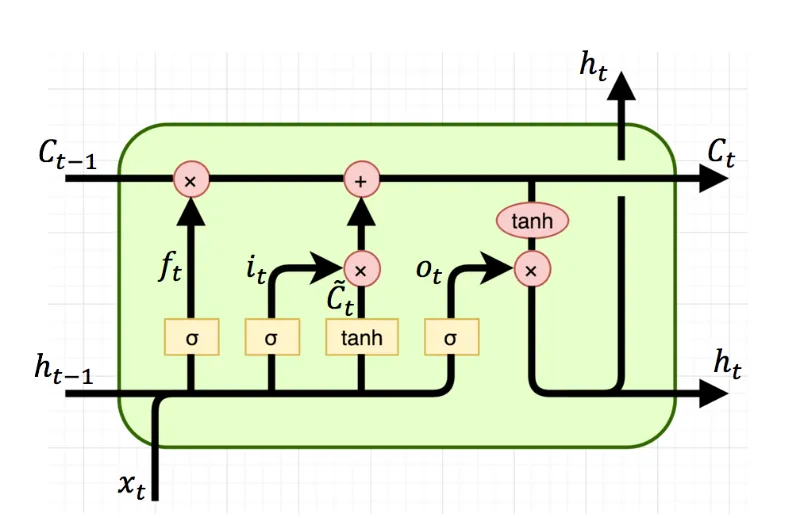
The LSTM cell consists of the following components: \[ \begin{aligned} f_t &= \sigma(W_{if}x_t + b_{if} \;+\; W_{hf}h_{t-1} + b_{hf}) \\ i_t &= \sigma(W_{ii}x_t + b_{ii} \;+\; W_{hi}h_{t-1} + b_{hi}) \\ o_t &= \sigma(W_{io}x_t + b_{io} \;+\; W_{ho}h_{t-1} + b_{ho}) \\ \tilde{c}_t &= \tanh(W_{ic}x_t + b_{ic} \;+\; W_{hc}h_{t-1} + b_{hc}) \\ c_t &= f_t \odot c_{t-1} + i_t \odot \tilde{c}_t \\ h_t &= o_t \odot \tanh(c_t) \end{aligned} \]

where \(f_t\), \(i_t\), and \(o_t\) are the forget, input, and output gates, respectively. \(\tilde{c}_t\) is the candidate memory state, \(c_t\) is the memory state, and \(h_t\) is the hidden state at time step \(t\). \(x_t\) is the input at time step \(t\), \(h_{t-1}\) is the hidden state at time step \(t-1\), and \(W\) and \(b\) are the weights and biases of each gate.

CIFG LSTM

In this post, we’ll implement a special of type of LSTM called Coupled Input and Forget Gate (CIFG) Greff et al. (2017). In CIFG LSTM, the input gate is computed as: \[i_t = 1 - f_t\] This reduces the number of parameters in the model and has been shown to perform well in practice.

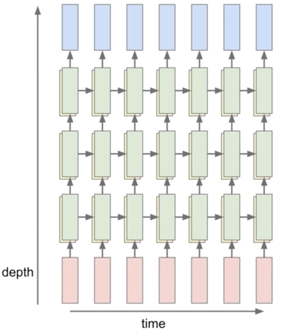
Multi-layers

A multi-layer LSTM is simply stacking multiple LSTM cells on top of each other. The output of the previous LSTM cell is fed as input to the next LSTM cell. The hidden state of the last LSTM cell is the input to the classification layer.

Multi-layer LSTM Example CS231n (2023). Each row of the green rectangles represent an LSTM cell.

Now let’s get into the implementation, step by step.

lstm.py

#

Import the dependencies.
The activation functions are defined in a separate module

1from collections import defaultdict
2from copy import deepcopy
3
4import numpy as np
5from op import sigmoid, softmax, tanh

#

LSTM Classifier

Multi-layer LSTM classifier for sequence classification tasks.

It consists of an embedding layer, multiple LSTM cells, and a classification head. The model is used to process input sequences and generate output logits.

6class LSTMClassifier:

#

• embed_size: Dimension of the word embeddings, or more generally, the input features.
• hidden_size: The size of the hidden state of the LSTM cells.
• vocab_size: The number of unique tokens in the vocabulary.
• n_cells: Number of stacked LSTM cells in the model.

 7    def __init__(
 8        self,
 9        embed_size: int,
10        hidden_size: int,
11        vocab_size: int,
12        n_cells: int = 1,
13    ) -> None:

#

Define internal variables

14        self.embed_size = embed_size
15        self.hidden_size = hidden_size
16        self.vocab_size = vocab_size
17        self.n_cells = n_cells
18        self.layers = dict()

#

Create embedding layer to convert word indices to embeddings

19        self.layers["embedding"] = np.empty((vocab_size, embed_size))

#

Create LSTM layers

20        for cell_index in range(n_cells):

#

For every forget, output, and cell gates, create a linear layer

21            for layer_name in ["f", "o", "c"]:

#

The input size of the first layer is embed_size + hidden_size, since the input is the concatenation of the input features and the previous hidden state. For subsequent layers, the input size is 2 x hidden_size.

22                linp_sz = hidden_size + (
23                    embed_size if cell_index == 0 else hidden_size
24                )

#

Weights and bias for the linear layer

25                self.layers[f"W{layer_name}_{cell_index}"] = np.empty(
26                    (linp_sz, hidden_size)
27                )
28                self.layers[f"b{layer_name}_{cell_index}"] = np.empty(
29                    (hidden_size)
30                )

#

Classification head (projection layer) to generate logits

31        self.layers["W_head"] = np.empty((hidden_size, vocab_size))
32        self.layers["b_head"] = np.empty((vocab_size))

#

Create the gradient arrays. These will be used to store the gradients during backpropagation.

33        self.grad = {k: np.empty_like(v) for k, v in self.layers.items()}

#

Initialize the weights

34        self.init_weights()

#

Calculate the total number of parameters in the model. The size property of a numpy array returns the number of elements in the array.

35    @property
36    def num_parameters(self):
37        return sum(l.size for l in self.layers.values())

#

Glorot/Xavier initialization

The weights are initialized from a uniform distribution in the range \([-d, d]\), where \(d = \sqrt{\frac{6.0}{(r + c)}}\), and \(r\) and \(c\) are the number of rows and columns in the weight matrix. This makes the variance of the weights inversely proportional to the number the units, and helps in preventing the gradients from vanishing or exploding during training. The biases are initialized to zero.

38    def init_weights(self):
39        for name, layer in self.layers.items():
40            if layer.ndim == 1:
41                self.layers[name] = np.zeros((layer.shape[0]))
42            elif layer.ndim == 2:
43                r, c = layer.shape
44                d = np.sqrt(6.0 / (r + c))
45                self.layers[name] = np.random.uniform(-d, d, (r, c))

#

Initialize the hidden and cell states for the LSTM layers.

46    def init_state(self, batch_size):
47        state = dict()

#

For every LSTM cell and every sample in the batch, initialize the hidden and cell states to zeros.

48        state["h"] = np.zeros((self.n_cells, batch_size, self.hidden_size))
49        state["c"] = np.zeros((self.n_cells, batch_size, self.hidden_size))
50        return state

#

Forward pass through the LSTM model.

• inputs: Input sequences of shape (batch_size, seq_len, features)
• state: Hidden and cell states of the LSTM layers. If None, initialize the states to zeros.
• teacher_forcing: If True, use inputs as the input at each timestep. If False, inputs is used as the prefix.
• generation_length: Length of the generated sequence when teacher_forcing is False.

51    def forward(
52        self, inputs, state=None, teacher_forcing=True, generation_length=0
53    ):
54        batch_sz, seq_len = inputs.shape[:2]
55
56        if teacher_forcing is True:
57            assert generation_length == 0
58
59        n_timestamps = seq_len + generation_length

#

Dictionary to store the activations at each timestep. This'll be used during backpropagation.

60        activations = defaultdict(lambda: defaultdict(list))

#

Output probabilities of every token in the vocabulary at each timestep

61        outputs = np.zeros((batch_sz, n_timestamps, self.vocab_size))

#

Initialize the hidden and cell states

62        if state is None:
63            state = self.init_state(batch_sz)
64        else:
65            state = state.copy()  # make a shallow copy
66        for k in ["h", "c"]:
67            activations[k][-1] = state[k]

#

Process the input sequences

68        for timestep in range(n_timestamps):

#

If teacher forcing is False and the prefix is consumed, use the previous prediction as the input for the next timestep

69            if teacher_forcing is False and timestep >= 1:
70                word_indices = np.argmax(outputs[:, timestep - 1], axis=1)
71            else:
72                word_indices = inputs[:, timestep]
73            features = self.layers["embedding"][word_indices]
74            activations["input"][timestep] = word_indices

#

Forward pass through the LSTM cells

75            for cell_idx in range(self.n_cells):

#

Previous cell states

76                h_prev = state["h"][cell_idx]
77                c_prev = state["c"][cell_idx]

#

We can simplify the gate operation by concatenating the input features with the hidden state, and perform a single linear projection instead of two.

78                X = np.concatenate((features, h_prev), axis=-1)

#

Apply the gates, which are linear operations followed by activation functions

\( \begin{aligned} f_t &= \sigma(W_{if}{input}_t + b_{if} \;+\; W_{hf}h_{t-1} + b_{hf}) \\[1ex] i_t &= 1 - f_t \qquad\qquad \text{Coupled forget and input gates} \\[1ex] o_t &= \sigma(W_{io}{input}_t + b_{io} \;+\; W_{ho}h_{t-1} + b_{ho}) \\[1ex] \tilde{c}_t &= \tanh(W_{ic}{input}_t + b_{ic} \;+\; W_{hc}h_{t-1} + b_{hc}) \\[1ex] \end{aligned} \)

79                f = sigmoid(
80                    X @ self.layers[f"Wf_{cell_idx}"]
81                    + self.layers[f"bf_{cell_idx}"]
82                )
83                i = 1 - f
84                o = sigmoid(
85                    X @ self.layers[f"Wo_{cell_idx}"]
86                    + self.layers[f"bo_{cell_idx}"]
87                )
88                c_bar = tanh(
89                    X @ self.layers[f"Wc_{cell_idx}"]
90                    + self.layers[f"bc_{cell_idx}"]
91                )

#

New memory cell and hidden state

\( \begin{aligned} c_t &= f_t \odot c_{t-1} + i_t \odot \tilde{c}_t \\[1ex] h_t &= o_t \odot \tanh(c_t) \end{aligned} \)

92                c = f * c_prev + i * c_bar
93                h = o * tanh(c)

#

Classification head

94                if cell_idx == self.n_cells - 1:
95                    logits = h @ self.layers["W_head"] + self.layers["b_head"]
96                    probs = softmax(logits, axis=1)
97                    outputs[:, timestep] = probs

#

Update the state for the next timestep

 98                state["c"][cell_idx] = c
 99                state["h"][cell_idx] = h
100                features = h

#

Save the activations for backpropagation

101                for k, v in zip(
102                    ["x", "f", "o", "c_bar", "c", "h"], [X, f, o, c_bar, c, h]
103                ):
104                    activations[k][timestep].append(v)

#

105        return outputs, state, activations

#

Alias for the forward method, similar to PyTorch's nn.Module. This enables model(inputs) \(\equiv\) model.forward(inputs)

106    __call__ = forward

#

Backward pass to compute the gradients.

• grad: Gradient of the loss with respect to the output of the model, i.e. logits (pre-softmax scores)
• activations: Activations from the forward pass.

107    def backward(self, grad, activations):
108        batch_sz, seq_len = grad.shape[:2]

#

Initialize the gradients of the next timestep to zeros. This will be updated as we move backward in time.

109        grad_next = {
110            k: np.zeros((self.n_cells, batch_sz, self.hidden_size))
111            for k in ["h", "c"]
112        }

#

Helper function to compute the gradients of the linear layer. The gradients are computed with respect to the input, weights, and biases respectively.

• X: Input to the linear layer
• W: Weights of the linear layer
• dY: Gradient of the loss with respect to the output of the linear layer

113        def _lin_grad(X, W, dY):
114            return (dY @ W.T, X.T @ dY, dY)

#

Backpropagation through time. Let's denote \(t\) as the current timestep

115        for timestep in reversed(range(seq_len)):

#

Classification head

116            dout_t = grad[:, timestep]
117            h = activations["h"][timestep][-1]

#

The gradients for the classification head: \(\text{logits}_t = h_t \mathbf{W}_{\text{head}} + \mathbf{b}_{\text{head}}\)

118            dh, dW_head, db_head = _lin_grad(
119                X=h, W=self.layers["W_head"], dY=dout_t
120            )
121            self.grad[f"W_head"] += dW_head
122            self.grad[f"b_head"] += np.sum(db_head, axis=0)

#

Iterate over the LSTM cells in reverse order

123            for cell_idx in reversed(range(self.n_cells)):

#

Get the activations for the current timestep

124                x, f, o, c_bar, c = (
125                    activations[key][timestep][cell_idx]
126                    for key in ["x", "f", "o", "c_bar", "c"]
127                )

#

Cell state from the previous timestep

128                c_prev = activations["c"][timestep - 1][cell_idx]

#

Receive the gradients flowing from the next timestep.
The gradient of the hidden state \(h_t\) is the sum of the gradients from the next cell and the next timestep.

129                dh += grad_next["h"][cell_idx]
130                dc = grad_next["c"][cell_idx]

#

\(h_t = o * tanh(c_t)\)

131                do = dh * tanh(c)
132                dc += dh * o * tanh(c, grad=True)

#

\(c_t = f_t \odot c_{t-1} + (1 - f_t) \odot \tilde{c}_t\)

133                df = dc * (c_prev - c_bar)
134                dc_prev = dc * f
135                dc_bar = dc * (1 - f)

#

Pre-activation gradients

136                dc_bar *= tanh(c_bar, grad=True)
137                do *= sigmoid(o, grad=True)
138                df *= sigmoid(f, grad=True)

#

f, o, c gates and the inputs X and \(h_{t-1}\)
Since all the gates are linear operations, the calculation will be similar

139                dinp, dh_prev = 0, 0
140                for gate, doutput in zip(["f", "o", "c"], [df, do, dc_bar]):
141                    dX, dW, db = _lin_grad(
142                        X=x, W=self.layers[f"W{gate}_{cell_idx}"], dY=doutput
143                    )
144                    self.grad[f"W{gate}_{cell_idx}"] += dW
145                    self.grad[f"b{gate}_{cell_idx}"] += np.sum(db, axis=0)
146                    dinp_gate, dh_prev_gate = (
147                        dX[:, : -self.hidden_size],
148                        dX[:, -self.hidden_size :],
149                    )

#

Accumulate the gradients for the input and the hidden state, since they are shared between the gates

150                    dinp += dinp_gate
151                    dh_prev += dh_prev_gate

#

Flow the gradients to the previous cell and previous timestep

152                dh = dinp
153                grad_next["c"][cell_idx] = dc_prev
154                grad_next["h"][cell_idx] = dh_prev

#

Embedding layer

155            word_indices = activations["input"][timestep]
156            self.grad["embedding"][word_indices] += dinp

#

Helper method to serialize the model state, similar to PyTorch's state_dict. The state dictionary contains the model configuration, weights, and gradients. It can be used to save and load the model.

157    @property
158    def state_dict(self):
159        return dict(
160            config=dict(
161                embed_size=self.embed_size,
162                hidden_size=self.hidden_size,
163                vocab_size=self.vocab_size,
164                n_cells=self.n_cells,
165            ),
166            weights=deepcopy(self.layers),
167            grad=deepcopy(self.grad),
168        )

#

169    @classmethod
170    def from_state_dict(cls, state_dict):
171        obj = cls(**state_dict["config"])
172        for src, tgt in zip(
173            [state_dict["weights"], state_dict["grad"]],
174            [obj.layers, obj.grad],
175        ):
176            for k, v in src.items():
177                tgt[k][:] = v
178        return obj

3 Activation and Loss Functions

The activation functions used in LSTM are the sigmoid, tanh (hyperbolic tangent), and softmax functions.

• Sigmoid is used to compute the gates, which are values between 0 and 1 that control the flow of information.
  
• tanh function is used to compute the candidate memory state.
  
• Softmax is used to compute the output probabilities.

The loss function used is the cross-entropy loss, which is suitable for classification tasks. Next token prediction is indeed a classification task where the model predicts the probability distribution over the vocabulary for the next token in the sequence.

op.py

#

Sigmoid function

The sigmoid squashes the input to the range [0, 1].

• If the flag grad is False, returns the sigmoid of x: $$\sigma(x) = \frac{1}{1 + e^{-x}}$$
• Otherwise, \(x = \sigma(z)\) and the derivate \(\frac{\partial \sigma(z)}{\partial z}\) is returned: $$\frac{\partial \sigma(z)}{\partial z} = \sigma(z) * (1 - \sigma(z))= x(1-x)$$.

1import numpy as np
2
3
4def sigmoid(x, grad=False):
5    if not grad:
6        return 1 / (1 + np.exp(-x))
7    return x * (1 - x)

#

Hyperbolic tangent function

The tanh function squashes the input to the range [-1, 1]. It's defined as: $$\tanh(x) = \frac{e^{x} - e^{-x}}{e^{x} + e^{-x}}$$

 8def tanh(x, grad=False):
 9    if not grad:
10        return np.tanh(x)
11    return 1 - x**2

#

Softmax function

Applies the softmax function to the input array along the specified axis. Softmax converts a vector of real numbers into a probability distribution. The logits are first exponentiated to make them positive and increase their separation. It's defined as: $$\text{softmax}(x_i) = \frac{e^{x_i}}{\sum_{j} e^{x_j}}$$

12def softmax(x, axis):

#

Subtracting the maximum value for numerical stability. Softmax is invariant to to a constant shift

13    exps = np.exp(x - np.max(x, axis=axis, keepdims=True))
14    return exps / np.sum(exps, axis=axis, keepdims=True)

#

Cross-entropy loss function

Computes the cross-entropy loss between the predicted and target distributions. The cross-entropy loss is defined as: $$H(y, p) = -\sum_{i} y_i \log(p_i)$$

• prediction: The predicted array of probabilities of shape (batch_size, num_classes).
• target: The target array of shape (batch_size,) containing the class indices.

15def cross_entropy(prediction, target, reduction="mean"):
16    eps = np.finfo(prediction.dtype).eps
17    prediction = np.clip(prediction, eps, 1 - eps)

#

Take the negative log of the predicted probability of the target class

18    loss = -np.take_along_axis(
19        np.log(prediction), target[..., np.newaxis], axis=-1
20    )

#

Aggregate the loss

21    if reduction == "mean":
22        loss = loss.mean()
23    elif reduction == "sum":
24        loss = loss.sum()
25    return loss

4 AdamW

AdamW is a variant of the Adam optimizer that decouples weight penalty from the optimization steps, where the weight penalty is applied directly to the gradients. Adam optimizer uses both the first and second moments of the gradients to adapt the learning rate tailored to each parameter. The benefit of Adam/AdamW is that it requires little tuning of hyperparameters compared to RMSprop and SGD. We’ll go over each step of the optimization in the implementation.

optim.py

#

Import NumPy

1import numpy as np

#

2class AdamW:

#

AdamW Optimizer

Parameters:

• params (dict): Dictionary referencing the model parameters
• grads (dict): Dictionary referencing the gradients of the model parameters
• lr (float): Learning rate
• betas (Tuple[float, float]): Coefficients used for computing running averages of gradient and its square
• eps (float): Term added to the denominator to improve numerical stability
• weight_decay (float): Weight decay (L2 penalty) coefficient
• amsgrad (bool): Whether to use the AMSGrad variant of the algorithm

 3    def __init__(
 4        self,
 5        params: dict,
 6        grads: dict,
 7        lr=0.001,
 8        betas: tuple[float, float] = (0.9, 0.999),
 9        eps: float = 1e-8,
10        weight_decay: float = 1e-2,
11        amsgrad: bool = False,
12    ):
13        self.params = params
14        self.grads = grads
15        self.lr = lr
16        self.betas = betas
17        self.eps = eps
18        self.weight_decay = weight_decay
19        self.amsgrad = amsgrad

#

Counter for the number of iterations

20        self.n_iters = 0

#

Initialize first moment vector (mean of gradients) for each parameter

21        self.m = {k: np.zeros_like(v) for k, v in params.items()}

#

Initialize second moment vector (uncentered variance of gradients) for each parameter

22        self.v = {k: np.zeros_like(v) for k, v in params.items()}

#

Initialize maximum of second moment vector for AMSGrad if needed

23        self.v_m = (
24            {k: np.zeros_like(v) for k, v in params.items()}
25            if amsgrad
26            else None
27        )

#

Resets all gradients to zero. This is typically used before computing new gradients in the training loop.

28    def zero_grad(self):
29        for v in self.grads.values():
30            v[:] = 0

#

Perform a single optimization step.

Updates the parameters of the model using the AdamW update rule, which includes bias correction, optional AMSGrad, and weight decay.

31    def step(self):

#

Increment the iteration counter

32        self.n_iters += 1

#

Unpack the beta values

33        beta1, beta2 = self.betas

#

Iterate over the parameters and their gradients

34        for (name, param), grad in zip(
35            self.params.items(), self.grads.values()
36        ):

#

Update the first moment estimate: $$m_t = \beta_1 \cdot m_{t-1} + (1 - \beta_1) \cdot g_t$$ where \(\beta_1\) is the exponential decay rate for the first moment estimates, and \(g_t\) is the gradient at time step \(t\).
\(m_{t}\) is simply an exponential moving average (EMA) of the past gradients.

37            m_t = self.m[name] = beta1 * self.m[name] + (1 - beta1) * grad

#

Update the second moment estimate: $$v_t = \beta_2 \cdot v_{t-1} + (1 - \beta_2) \cdot g_t^2$$ where \(\beta_2\) is the exponential decay rate for the second moment estimates.

38            v_t = self.v[name] = beta2 * self.v[name] + (1 - beta2) * (
39                grad**2
40            )

#

Compute bias-corrected first moment estimate: $$\hat{m}_t = \frac{m_t}{1 - \beta_1^t}$$

Without correction, the bias causes the algorithm to move very slowly at the beginning of training, as the moment estimates are underestimated. In the early iterations, \(t\) is small, so \(\beta_1^t\) is close to 1, making \(1 - \beta_1^t\) a small number. Dividing by this small number effectively increases the estimate.

41            m_t_hat = m_t / (1 - beta1**self.n_iters)

#

Compute bias-corrected second moment estimate: $$\hat{v}_t = \frac{v_t}{1 - \beta_2^t}$$

42            v_t_hat = v_t / (1 - beta2**self.n_iters)

#

AMSGrad update: $$\hat{v}_t = \max(\hat{v}_t, v_{t-1})$$ where \(v_{t-1}\) is the previous second moment estimate. This ensures \(v_t\) is always non-decreasing, preventing the learning rate from growing too large.

43            if self.amsgrad:
44                v_t_hat = self.v_m[name] = np.maximum(self.v_m[name], v_t_hat)

#

Adjusted gradient: $$\hat{g} = \frac{\hat{m}_t}{\sqrt{\hat{v}_t} + \epsilon}$$ where \(\epsilon\) is a small constant to avoid division by zero.
\(\frac{\hat{m}_t}{\sqrt{\hat{v}_t}}\) can be thought of as the signal-to-noise ratio of the gradient. I'll leave the intuition behind this to another blog post.

45            g_hat = m_t_hat / (np.sqrt(v_t_hat) + self.eps)

#

Add weight penalty to the update: $$\text{update} = \hat{g} + \lambda \cdot p$$ where \(\lambda\) is the weight_decay coefficient. This is equivalent to adding the L2 penalty to the loss function, which penalizes large weights.

46            update = g_hat + self.weight_decay * param

#

Update the parameters in the direction of the negative gradient, scaled by the learning rate: $$ p_t = p_{t-1} - \eta \cdot \text{update}$$ where \(p_{t-1}\) is the previous parameter value.

47            self.params[name] -= self.lr * update

5 Data Utilities

In this section we’ll implement the Dataset and Dataloader classes to handle the Shakespeare dataset. We follow the best practices of PyTorch’s Dataset and DataLoader classes to make the implementation more modular and reusable.

• The Dataset class implements the __getitem__ method, which returns a single sample from the dataset.
• The DataLoader class will be used to sample mini-batches from the dataset, by calling the __getitem__ method of the Dataset.

data.py

#

Import NumPy

1import numpy as np

#

Dataset

A dataset for next character prediction tasks.

For a sequence of characters \([c_1, c_2, ..., c_n]\) and a given sequence length \(l\), this dataset creates input/target pairs of the form:

• Input \(x_i\): \([c_i, c_{i+1}, ..., c_{i+l-1}]\)
• Target \(y_i\): \([c_{i+1}, c_{i+2}, ..., c_{i+l}]\)

where \(i\) ranges from 1 to \(n-l\).

Each item in the dataset is a tuple \((x_i, y_i)\) where both \(x_i\) and \(y_i\) have length \(l\). The task is to predict each character in \(y_i\) given the corresponding prefix in \(x_i\).

For example, given \(x_i = [c_i, c_{i+1}, c_{i+2}]\), the model would aim to predict:

• \(c_{i+1}\) given \([c_i]\)
• \(c_{i+2}\) given \([c_i, c_{i+1}]\)
• \(c_{i+3}\) given \([c_i, c_{i+1}, c_{i+2}]\)

2class NextCharDataset:

#

3    def __init__(self, data, seq_length):
4        self.data = data.copy()

#

Create a sliding window view of the data

5        self.window_view = np.lib.stride_tricks.sliding_window_view(
6            self.data, window_shape=seq_length + 1
7        )

#

8    def __len__(self):
9        return len(self.window_view)

#

\(\text{Input}_i\): \([c_i, c_{i+1}, ..., c_{i+l-1}]\)

\(\text{Target}_i\): \([c_{i+1}, c_{i+2}, ..., c_{i+l}]\)

10    def __getitem__(self, idx):
11        x, y = self.window_view[idx, :-1], self.window_view[idx, 1:]
12        return x, y

#

DataLoader

A simple DataLoader to iterate over a dataset in batches.

13class DataLoader:

#

14    def __init__(self, dataset, batch_size, shuffle=False, drop_last=False):
15        self.dataset = dataset
16        self.batch_size = batch_size
17        self.shuffle = shuffle
18        self.drop_last = drop_last

#

The __iter__ method returns an iterator that yields batches of data. It's mainly used in a for loop to iterate over the dataset. e.g.:

for inputs, targets in dataloader:
    ...

19    def __iter__(self):
20        indices = np.arange(len(self.dataset))
21
22        if self.shuffle:
23            np.random.shuffle(indices)
24
25        if self.drop_last:
26            remainder = len(self.dataset) % self.batch_size
27            if remainder:
28                indices = indices[:-remainder]
29
30        for i in range(0, len(indices), self.batch_size):
31            batch_indices = indices[i : i + self.batch_size]
32            batch = [self.dataset[j] for j in batch_indices]
33            yield self.collate_fn(batch)

#

34    def __len__(self):
35        if self.drop_last:
36            return len(self.dataset) // self.batch_size
37        else:
38            return np.ceil(len(self.dataset) / self.batch_size).astype(int)
39
40    def collate_fn(self, batch):
41        if isinstance(batch[0], (tuple, list)):
42            return [np.array(samples) for samples in zip(*batch)]
43        elif isinstance(batch[0], dict):
44            return {
45                key: np.array([d[key] for d in batch]) for key in batch[0]
46            }
47        else:
48            return np.array(batch)

6 Training on Shakespeare dataset

Now it’s time to put everything together and train the model on the a dataset. We’ll use the Shakespeare dataset, which consists of a collection of Shakespeare’s plays. The model will be trained to predict the next character in the sequence given a sequence of characters.

An important distinction to make between the text generation at training time and inference time is that at training time, we feed the ground truth characters to the model to predict the next character; This is called teacher forcing. At inference time, we feed the model’s prediction at time step \(t\) as the input at time step \(t+1\) to predict the next character.

6.1 Load

import numpy as np
import matplotlib.pylab as plt

Download the Shakespeare dataset which is a single text file from the following link: Shakespeare dataset

with open("shakespeare.txt") as file:
    data = file.read()

print(data[:200])

First Citizen:
Before we proceed any further, hear me speak.

All:
Speak, speak.

First Citizen:
You are all resolved rather to die than to famish?

All:
Resolved. resolved.

First Citizen:
First, you

6.2 Preprocess

We need to convert the text data into numerical data. Using scikit-learn’s LabelEncoder we can map each character to a unique integer. The same encoder will be used to inverse transform the predictions back to characters.

from sklearn.preprocessing import LabelEncoder

char_data = np.array(list(data))
encoder = LabelEncoder()
indices_data = encoder.fit_transform(char_data)

vocabulary = encoder.classes_
vocabulary

array(['\n', ' ', '!', '$', '&', "'", ',', '-', '.', '3', ':', ';', '?',
       'A', 'B', 'C', 'D', 'E', 'F', 'G', 'H', 'I', 'J', 'K', 'L', 'M',
       'N', 'O', 'P', 'Q', 'R', 'S', 'T', 'U', 'V', 'W', 'X', 'Y', 'Z',
       'a', 'b', 'c', 'd', 'e', 'f', 'g', 'h', 'i', 'j', 'k', 'l', 'm',
       'n', 'o', 'p', 'q', 'r', 's', 't', 'u', 'v', 'w', 'x', 'y', 'z'],
      dtype='<U1')

An example of the mapped data:

indices_data[:200]

array([18, 47, 56, 57, 58,  1, 15, 47, 58, 47, 64, 43, 52, 10,  0, 14, 43,
       44, 53, 56, 43,  1, 61, 43,  1, 54, 56, 53, 41, 43, 43, 42,  1, 39,
       52, 63,  1, 44, 59, 56, 58, 46, 43, 56,  6,  1, 46, 43, 39, 56,  1,
       51, 43,  1, 57, 54, 43, 39, 49,  8,  0,  0, 13, 50, 50, 10,  0, 31,
       54, 43, 39, 49,  6,  1, 57, 54, 43, 39, 49,  8,  0,  0, 18, 47, 56,
       57, 58,  1, 15, 47, 58, 47, 64, 43, 52, 10,  0, 37, 53, 59,  1, 39,
       56, 43,  1, 39, 50, 50,  1, 56, 43, 57, 53, 50, 60, 43, 42,  1, 56,
       39, 58, 46, 43, 56,  1, 58, 53,  1, 42, 47, 43,  1, 58, 46, 39, 52,
        1, 58, 53,  1, 44, 39, 51, 47, 57, 46, 12,  0,  0, 13, 50, 50, 10,
        0, 30, 43, 57, 53, 50, 60, 43, 42,  8,  1, 56, 43, 57, 53, 50, 60,
       43, 42,  8,  0,  0, 18, 47, 56, 57, 58,  1, 15, 47, 58, 47, 64, 43,
       52, 10,  0, 18, 47, 56, 57, 58,  6,  1, 63, 53, 59])

6.3 Initialize

Now let’s define the dataloader, the model and the optimizer. I used the following hyperparameters below, but feel free to experiment with different values.

SEQUENCE_LENGTH = 128
BATCH_SIZE = 32
VOCAB_SIZE = len(vocabulary)
TRAIN_SPLIT = 0.8
LEARNING_RATE = 0.001
SHUFFLE_TRAIN = True

EMBED_SIZE = 256
HIDDEN_SIZE = 512
NUM_LAYERS = 2
NUM_EPOCHS = 5

Define the train and test data loaders

from data import NextCharDataset, DataLoader

trainset_size = int(len(indices_data) * TRAIN_SPLIT)
train_data = indices_data[:trainset_size]
test_data = indices_data[trainset_size:]

trainset = NextCharDataset(train_data, SEQUENCE_LENGTH)
testset = NextCharDataset(test_data, SEQUENCE_LENGTH)

trainloader = DataLoader(trainset, batch_size=BATCH_SIZE, shuffle=SHUFFLE_TRAIN)
testloader = DataLoader(testset, batch_size=BATCH_SIZE, shuffle=False)

Define the model and optimizer

from lstm import LSTMClassifier
from optim import AdamW

model = LSTMClassifier(EMBED_SIZE, HIDDEN_SIZE, VOCAB_SIZE, NUM_LAYERS)
optimizer = AdamW(params=model.layers, grads=model.grad, lr=LEARNING_RATE)

6.4 Training loop

The training loop follows this standard structure:

for epoch = 1 to TOTAL_EPOCHS:    
    // Training Phase
    for each batch in train_data:
        predictions = forward_pass(model, batch)
        loss = compute_loss(predictions, true_labels)
        gradients = compute_gradients(loss)
        update_model_parameters(model, gradients)
        record_metrics(loss, accuracy, ...)
    
    // Testing Phase
    for each batch in test_data:
        predictions = forward_pass(model, batch)
        loss = compute_loss(predictions, true_labels)
        record_metrics(loss, accuracy, ...)

Most of the implementation such as the forward and backward passes, optimization and data loading is already done. The remaining part is loss computation and gradient of loss w.r.t the predictions. Since next-token prediction is a classification task, we’ll use the cross-entropy loss function.

from tqdm.auto import tqdm
from collections import defaultdict
from op import cross_entropy

state = None
train_losses = defaultdict(list)
test_losses = defaultdict(list)

for epoch in tqdm(range(NUM_EPOCHS), desc="Epoch"):
    # training loop
    for inputs, targets in (pbar := tqdm(trainloader, leave=False)):
        if SHUFFLE_TRAIN:
            state = None
        probabilities, state, activations = model.forward(inputs, state)

        # cross entropy loss
        loss = cross_entropy(probabilities, targets)
        # accuracy
        accuracy = np.mean(np.argmax(probabilities, axis=-1) == targets)

        # loss gradient w.r.t logits (before softmax)
        gradient = np.copy(probabilities)
        # Subtract 1 from the probabilities of the true classes
        # Since the gradient is p_i - y_i
        gradient[np.arange(targets.shape[0])[:, None], 
                 np.arange(targets.shape[1]), targets] -= 1
        # Subtract 1 from the probabilities of the true classes
        gradient /= gradient.shape[0]

        # backpropagate and update
        optimizer.zero_grad()
        model.backward(gradient, activations)
        optimizer.step()

        # log
        pbar.set_postfix({"loss": f"{loss:.5f}", 
                          "accuracy": f"{accuracy*100:.2f}"})
        train_losses[epoch].append(loss)

    # testing loop
    loss_sum = 0
    accuracy_sum = 0
    for iter, (inputs, targets) in (pbar := tqdm(enumerate(testloader),
                                                 leave=False)):
        probabilities, state, _ = model.forward(
            inputs, state=None, teacher_forcing=False
        )
        loss = cross_entropy(probabilities, targets)
        accuracy = np.mean(np.argmax(probabilities, axis=-1) == targets)

        loss_sum += loss
        accuracy_sum += accuracy
        pbar.set_postfix(
            {
                "loss": f"{loss_sum / (iter + 1):.5f}",
                "accuracy": f"{accuracy_sum / (iter + 1)*100:.2f}",
            }
        )
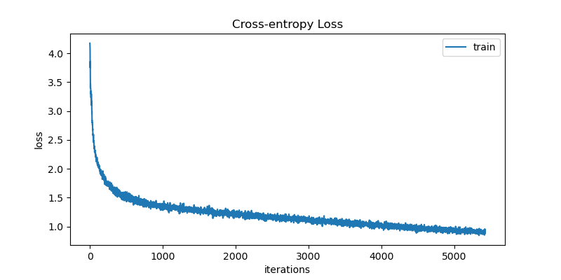
        test_losses[epoch].append(loss)

Now that it’s time for training, the bad news is that the process will be slow! Understandably so, since we’re using NumPy over CPU. Still, I trained the model for ~6000 iterations (batches) to make sure the implementation is correct and that the model is learning. The figure below shows the loss curve decreasing consistently over the iterations.

Training Loss Curve

For checkpointing, we can save the model to disk:

np.save("checkpoint.npy", model.state_dict)

To reload from the checkpoint, use the from_state_dict method:

state_dict = np.load("checkpoint.npy", allow_pickle=True).item()
model = LSTMClassifier.from_state_dict(state_dict)

state_dict.keys()

dict_keys(['config', 'weights', 'grad'])

6.5 Generating text

At inference time, we feed the model a prefix text and let it generate the next characters. We can control the number of characters to generate by setting the generate_length parameter in forward. I used greedy decoding to generate the text which works by selecting the character with the highest probability at each time step.

def generate(model, prefix: str, length: int):
    inputs = np.array(list(prefix))
    inputs = encoder.transform(inputs)
    inputs = inputs[np.newaxis]
    state = None

    probabilities, state, _ = model.forward(
        inputs, state, teacher_forcing=False, generation_length=length
    )
    tokens = np.argmax(probabilities[0, len(prefix) - 1 :], axis=-1)

    output = prefix + "".join(encoder.inverse_transform(tokens))
    return output

print(generate(model, prefix="I will", length=400))

I will rest blood that bear blood at all,
And stay the king to the consulships?

MENENIUS:
Nay, then he will stay the king to the cause of my son's exile is banished.

ROMEO:
And stay the common people: there is no need, that I may call thee back.

NORTHUMBERLAND:
Here comes the county strict ready to give me leave to see him as he fall be thine, my lord.

KING RICHARD II:
Norfolk, throw down the coronat

Looks like the model was able to learn something! As an alternative to basic sampling, more advanced techniques like beam search, Top-K sampling, and nucleus sampling can significantly enhance the text generation quality but that’d be beyond the scope of this post.

I hope you found this post helpful. If you have any questions or suggestions, feel free to leave a comment. Thanks for reading!

References

[1]

CS231n. Convolutional neural networks for visual recognition, https://cs231n.github.io/rnn/, 2023.

[2]

Klaus Greff, Rupesh K. Srivastava, Jan Koutnik, Bas R. Steunebrink, and Jurgen Schmidhuber. LSTM: A search space odyssey, IEEE Transactions on Neural Networks and Learning Systems, vol. 28, no. 10, 2222–2232, 2017. doi: 10.1109/tnnls.2016.2582924.

[3]

Christopher Olah. Understanding LSTM networks, https://colah.github.io/posts/2015-08-Understanding-LSTMs/, 2015.